Optimize N1QL performance using request profiling

Monitoring uncovered the resource hog. Now what?

Couchbase Server 4.5 introduced a mechanism to keep an eye on executing requests, so that slow performers could be highlighted.

This DZone article covers the subject of N1QL monitoring in great detail, but the question now is – we have the rioters, how do we check their demands?

In general terms, every database engine provides means to analyse the query plan used by a request to return data, in the form of some sort of EXPLAIN statement, but this does exactly what the word says: it explains the plan, but it does not actually say what part of the plan is misbehaving, using hard numbers.

Experienced database administrators can tell, using a mixture of, well, experience, heuristics and gut feelings how a specific plan could be improved, but this specific skill set requires a substantial amount of training, and, to be fair, a certain degree of guesswork is involved too.

Can we do better?

Enter profiling

Couchbase 5.0 introduces, among other things, the ability to collect metrics on all moving parts of individual requests.

When the feature is enabled, profiling information is returned by the request following the results document, and it is available in system keyspaces for later processing.

This metric shows the execution tree in detail, with such information as the time spent in each operator an and in each processing phase, as well as the documents ingested and digested.

Armed with this trove of data, database administrators can easily identify the costly operators in a request and address the problem, for example, creating the right index to minimize the number of qualified keys returned by the index scan.

But let’s start from the beginning.

Enabling profiling

The more frequent use of profiling is to understand why a particular statement is slow.

As such, the slow statement has already been identified and it is probably being tested in a sandbox environment – the only information needed is the culprit statement text and there’s no need to collect profiles from anything else.

Conversely, a production node may be  going through a slow patch.

The culprit request has not been identified and it is important to collect all available diagnostic information immediately so that once the slow request is identified, the profiling is already available without having to rerun the offending statement.

At the request level

This can be done with the profile request REST API parameter, passed to the query service alongside the request statement – ideal for investigating individual statements.

This could be down at the lowest possible level, as exemplified by this curl example

Or more simply from a cbq shell session

Query Workbench enables profiling by default as we will see later.

The profile parameter takes three values: off (the default), phases, and timings.

The first, as expected, just disables the feature.

The second enables a summary of execution timings for each request phase, while the last offers the highest level of information available: full timings on a per execution operator basis.

At the service level

When profiling is required across all requests, it can be enable at node startup via the -profile command line parameter.

This takes the same arguments as the query REST API parameter, with the same meaning.

Any request that does not specify any profiling level at the REST API level takes the value of the command line argument as the selected option.

On the fly

When production clusters are showing signs of fatigue, it is possible to change query service profile setting on the fly via the /admin/settings REST endpoint, as an example

This has the same effect as initializing the query service using the -profile command line parameter, however it also applies to requests that have already started, meaning that when the requests does not specify a query level profile setting, it will take the newly set level as the selected option.

It is important to know that profiling information is collected at all times – the switches above merely determine if and how much information is reported.

It is therefore possible to retroactively turn on profiling for requests that had already started, meaning that when noticing a system slowdown, a DBA can profile all already running requests, without having to resubmit any of the requests or investigate first which one is mis-performing!

Obtaining profiling information

Individual request profiling information is made available as a json subdocument detailing the execution tree.

In general terms, this is a structure in the same format and very close contents  as the EXPLAIN statement output, but augmented with execution statistics.

This can be accessed by the client application, via the response document (which is useful for one off investigations), and third parties, via the system keyspaces, which is useful for instance to compare different variations on the same statement, or execution of the same statement with different values for placeholders.

From the request response

The following example shows the execution of a statement in cbq, with profiling turned on

Note that the response now includes a profile section, showing phase information such as phaseTimes, phaseCounts, phaseOperators (respectively the time spent executing each phase, the number of documents processed per phase, and the number of operators executing each phase) – the only information provided when profile is set to phases – as well as an executionTimings subsection.

From system keyspaces

Queries on system keyspaces can return request profiling information, provided profiling is turned on for said requests at the time of the query.

Here’s a quick example:

The record for the select on system:active_requests itself is sporting phase information.

If profiling is set to timings, the detailed execution tree is reported as the plan attachment, accessible via the meta() function:

The information shown here in system:active_requests is also accessible from system:completed_requests, assuming that the request in question, on completion, qualifies for storage in system:completed_requests and profiling was turned on.

Note that the timing information returned by system:active_requests is current, meaning that it includes the execution timings accrued up to now: a second select on system:active_requests can therefore be used to determine the cost of a particular operator in the interval of time elapsed between the two selects.

Information provided

As shown in the following example

the execution tree document reports, for each operator, the number of documents ingested and digested (#itemsIn and #itemsOut), time spent executing operator code (execTime), waiting to be scheduled (kernTime) and waiting for services to supply data (servTime), the number of times the operator has changed state (executing, waiting to be scheduled, waiting for data), and the current state (assuming that the request has not already completed).

The operator statistics are purposely very detailed in nature: each individual measure has been known to stand out prominently during specific performance investigations, and I am not ashamed to say that they have also been gainfully used during my own debugging sessions!

To give a feeling of the sort of things that can be achieved, let’s consider phaseSwitches.

Suppose that, after gathering profiles twice, the number of phaseSwitches for a particular operator has not increased.

That particular operator may not be operating correctly: should the state be stuck in “services”, then depending on the operator, it may be waiting on the document store (for a Fetch), or the indexing service (for a Scan).

Maybe the relevant service is down or stuck?

Conversely, if stuck in “kernel”, then maybe a consumer down the pipeline is not accepting data, or the machine might be so loaded that the scheduler is not actually finding time slices for the operator.

The next section will cover some tell tale signs of some common scenarios, most likely scenarios first.

Interpreting profiles

Any operator: high kernel time

This is a bottleneck in an operator further down the pipeline.

Look for an operator with high execution or services time.

If one can’t be found, the runtime kernel is struggling to schedule operators: the query node is overloaded and adding a new one might come handy.

Fetches, Joins, Scans: high service times

This may indicate a stressed outside service.

A confirmation of this would come from a low rate of change in #itemsOut, although this requires taking the same profile more than once, which may be inconvenient (or impossible, if the request has already completed).

As an alternative, look for the symptoms described next.

Fetches and Joins: high service time per incoming document

Individual document fetches should be fast.

Dividing servTime by #itemsOut should always yield Fetch times of substantially less than a millisecond.

If it isn’t, then the document store is under stress.

To be clear – it isn’t necessarily the request being profiled that’s putting the store under stress: more likely than not it is the overall load on the service that’s being the issue.

One way to ascertain that overall load is the issue, at least, while performing stress tests, is just to reduce the number of worker clients: on an overloaded store, individual fetch times stay constant as the number of clients goes down, and only start to improve when the load gets to level that can be more easily handled.

Fetches: high number of documents ingested

A good query plan should use an index that produces only the document keys that are relevant for the request.

If the number of keys passed to the Fetch operator is much more than the final number of documents returned to the client, the index chosen in not selective enough.

Scans: high number of document produced

This is the counterpart of the previous symptom: the index chosen in not selective enough. Consider creating an index so additional predicates can be pushed to the index scan.

Joins: low ingested documents, high documents produced

Again, definitely a wrong index path: is the join supposed to produce so many results in the first place?

Filters: high ingested documents, low documents produced

Another “index chosen definitely not selective enough” indicator.

Filters: high execution time

This should never happen, and if it does, it’s more likely than not accompanied by the previous symptom.

Not only was the index not selective enough and returning too many document keys, but evaluating all the expressions in the WHERE clause for so many documents is proving to be rather expensive!

Projection: high execution time

Again, an unlikely one: the query service is struggling to assemble the result documents for the request.

How many terms do you have in the SELECT statement’s projection clause? Shave a few!

Do you have complex expressions?

Stream: high execution time

The request is struggling to convert the result in JSON form and send it to the client.

The pretty REST parameter may have been set to true in error.

The projection list may have too many terms.

Alternatively, there is a network problem, or the result documents being sent are way too large for the network to cope.

Controls

Many times, request behaviour is dependent on placeholder values, therefore it would be very useful to capture placeholder values alongside profiles.

This can be done with the controls query REST API, command line parameter and /admin/settings REST endpoint, which takes a true or false value.

Its behaviour is exactly the same as the profile setting, and can be set on a per request basis, at start up, on the fly, service wide – this too being retrospectively applied to running requests that hadn’t specified a setting.

Named and positional parameters will be reported in the request output in their own control section:

as well as in system keyspaces (although, unlike profiles, there’s no need to access any attachment via the meta() function):

Visual profiles

A rather easy way to access detailed profiling information for individual statements, without having to do anything special, is through the Query tab in the Admin Console UI.

Query WorkBench turns profiling on by default, and upon completion of the request, timings and document counts are readily available in pictorial form, by clicking on the “plan” button.

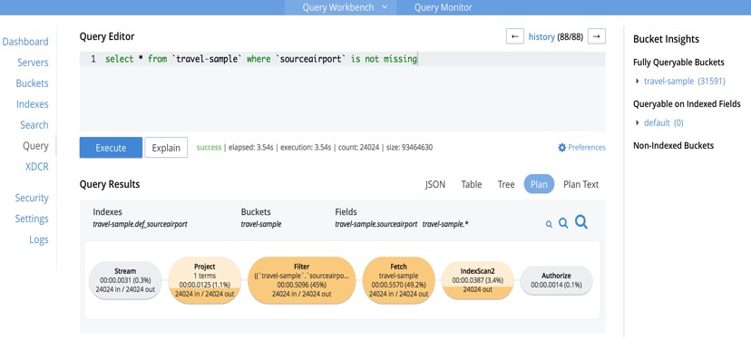
The operators are neatly colour coded by cost, and hovering over individual operators will result in copious amounts of raw timings popping up.

The Preferences allows to change profiling settings, as well as other settings such as named and positional parameters.

Profiling is much more than just profiling

Profile and controls information can be used for more detailed monitoring as well.

For instance, to find requests with any operator producing excessive amounts of documents, one could use

(change the threshold for output documents as required).

The example is quite simplistic, and could actually be more easily done using phaseCounts, but switch the ANY clause to satisfying

and presto!, the requests loading a specific keyspace are revealed.

Similarly, finding any request that used a specific value for any named parameter can be achieved with

(substitute “some parameter” and “target value” with the required values!)

The possibilities are endless.

One last consideration

Profiling information is held in the execution tree itself, which does use a fair amount of memory.

This in itself is not a problem, however, be mindful that when a slow running request becomes eligible for storage in system:completed_requests and profile is set to timings, the whole execution tree will be stored as well.

This, again, is not a problem in itself. It may become a problem, though, if system:completed_requests is set to log all requests, it has no limit, and all requests have profile set to timings: in this case, memory usage may grow beyond what is reasonable, because you are storing all timings for all requests ever executed since the beginning of time!

Happily, the default settings for system:completed_requests logging mean that you will not unknowingly land into trouble, and, anyway, I am not suggesting you should be thrifty with the amount of timings you log, but this is a case in which excess may be painful.

You have been warned.

Conclusions

Starting from Couchbase Server version 5.0, N1QL offers specialised tools to slice and dice execution timings in considerable depth.

Examples have been given on how to access the functionality and interpret the data collected.