
This post illustrates the use of Couchbase Analytics with the Couchbase Go SDK. Couchbase Analytics is a new service available in Couchbase Server 6.0, you can read more at https://docs.couchbase.com/server/6.0/analytics/introduction.html.
In this post we’re going to use a real world dataset which is big enough to not fit in memory (on my local machine at least). We’ll be using the CSV export of the 2016 NYC green taxi journey dataset. This is a dataset of ~16.4 million records with 23 fields per record. You can follow along and try out the application by cloning the project here, or run
go get github.com/chvck/gocb-taxi-analytics . You’ll also need to run
go get ./... if you’ve git cloned the project.
As this data is a CSV file the first job is to import it. Unfortunately this dataset uses non-standard datetime formats so we need to use a small script to go through and convert them into something more useable. If you’ve cloned the project then you can do this with
|
1 |
go run main.go --reformat --csv /path/to/taxis.csv |
This will create a
2016_Green_Taxi_Trip_Data.csv file in the project directory. I’ve also taken this opportunity to change the CSV headers to make them more JSON friendly and also add a type field always set to green (in case we later wanted to add the yellow taxi dataset too). During the conversion we could have also imported the data but we already have a great tool in cbimport that we can use. Create a bucket named taxis with full eviction enabled (under Advanced bucket settings – we won’t be running k/v operations so k/v performance does not matter as much in this instance) and then run:
|
1 |
cbimport csv --cluster couchbase://localhost -u user -p password -b taxis --infer-types -omit-empty -d file:///path/to/2016_Green_Taxi_Trip_Data.csv -l import.log -g green::%vendorID%::#MONO_INCR# |
Each document will have a unique ID like
green::1::1000 . Ordinarily these 2 steps wouldn’t be required as our data would already be held in Couchbase.
Before you can do any work with Couchbase Analytics you have to prepare a dataset to enable you to query the data:
|
1 |
CREATE DATASET alltaxis ON taxis; |
This dataset does require some resources. If you want to experiment with a slightly smaller dataset on a busy laptop, instead, you can make a filtered dataset which will only track a subset of the documents in your bucket:
|
1 |
CREATE DATASET alltaxis ON taxis WHERE `vendorID` = 1; |
This will you give you a dataset of a little over 3 million documents.
Once you’ve created one of the datasets then you need to initialise it by activating dataset processing with:
|
1 |
CONNECT LINK Local; |
This will begin populating the dataset that you’ve just created. You can see the progress in the UI in the right hand Datasets column, below the dataset name. You can continue to work with the dataset whilst it’s building but you’ll see different results each time that you run a query and execution may be a little slower.
As we’re going to be doing some data analysis it’s worth working out a couple of things to investigate. I think that a good starting point would be to know the number of taxi rides across the year and to be able to apply various filters to see things like tips against fares.
The base that we will use for our queries is:
|
1 |
SELECT DATE_PART_STR(pickupDate, "month") AS period, COUNT(*) as count FROM alltaxis GROUP BY DATE_PART_STR(pickupDate, "month") ORDER BY period; |
This query is extracting the month as a number (1-12) from the pickupDate field and displaying the number of journeys against the month. What we can see by running this query is that March has the most journeys and that November has the least journeys. There is also a downward trend across the year. I had expected Summer to have fewer journeys than the rest of the year so I’ve learned something already!
This query takes about 24s for the full dataset on my machine. Running the same against the operational query service (often just referred to as N1QL, but that’s the language) with only a primary index times out from the query console (600s). We can see that for ad hoc queries on large datasets Couchbase Analytics is a good option, complementing the operational N1QL query service .
Querying from a Golang Application
Now that we’ve setup and tested that our Analytics dataset works we can use it via the Go SDK. In the runServer function we have:
|
1 2 3 4 5 6 7 8 9 10 11 12 13 14 15 16 17 18 19 20 21 22 23 24 25 26 27 28 29 30 31 |
var err error cluster, err = gocb.Connect(cbConnStr) if err != nil { panic("Error connecting to cluster:" + err.Error()) } cluster.Authenticate(gocb.PasswordAuthenticator{ Username: cbUsername, Password: cbPassword, }) _, err = cluster.OpenBucket("taxis", "") if err != nil { log.Fatal(err) } stop := make(chan os.Signal, 1) // Stop the server on interrupt signal.Notify(stop, os.Interrupt) srv, err := run() if err != nil { log.Fatal(err) } fmt.Println("Server running on", srv.Addr) <-stop log.Println("Stopping server") srv.Shutdown(nil) |
This creates a connection to Couchbase Server and authenticates using the username and password (these properties can be customised by modifying the properties at the top of the main.go). Next we open a connection to our bucket. The remainder of the function is handling the web server. We create a channel listening to the interrupt signal and when that triggers we gracefully shutdown the http server.
It’s difficult to visualise and filter this data on the command line so in the linked codebase we’ve added a simple graphical UI. The web server serves up the index page and exposes a single endpoint for retrieving dynamic data. Once again, to run this use
go run main.go and you can access the frontend from
http://localhost:8010 .
Our handler for the dynamic data endpoint looks like this:
|
1 2 3 4 5 6 7 8 9 10 11 12 13 14 15 16 17 18 19 20 21 22 23 24 25 26 27 28 29 30 31 32 33 34 35 36 37 |
func requestHandler(w http.ResponseWriter, r *http.Request) { opts, err := processQueryString(r.URL.Query()) if err != nil { http.Error(w, err.Error(), http.StatusInternalServerError) return } q := `select DATE_PART_STR(pickupDate, "%s") AS period, %s as aggregate FROM alltaxis` q += ` %s GROUP BY DATE_PART_STR(pickupDate, "%s") ORDER BY period;` q = fmt.Sprintf(q, opts.Period, opts.Aggregate, opts.Where, opts.Period) query := gocb.NewAnalyticsQuery(q) results, err := cluster.ExecuteAnalyticsQuery(query, opts.Params) if err != nil { http.Error(w, err.Error(), http.StatusInternalServerError) return } data, err := processResults(results) if err != nil { http.Error(w, err.Error(), http.StatusInternalServerError) return } data.Where = fmt.Sprintf("%s %s, %v", opts.Aggregate, opts.Where, opts.Params) data.Query = fmt.Sprintf("query = %s, params = %v", q, opts.Params) data.TimeTaken = results.Metrics().ExecutionTime.Nanoseconds() js, err := json.Marshal(*data) if err != nil { http.Error(w, err.Error(), http.StatusInternalServerError) return } w.WriteHeader(200) w.Header().Set("Content-Type", "application/json") w.Write(js) } |
What we can see here is that we process the query string to extract the where (plus parameters, more on that below), aggregate and time period. We create our query as a string, incorporating these properties and then use NewAnalyticsQuery to create an AnalyticsQuery . To execute the query it is passed into cluster.ExecuteAnalyticsQuery . The results are then processed by processResults before sending the http response. Where , TimeTaken and Query properties are also added to the response so that we can display what’s been queried in the frontend.
Let’s look at each of these parts in a bit more detail. The where and aggregate parameters are passed from the frontend already formatted correctly. The query string could look something like
?period=hour&month=5&day=14&aggregate=count(*)&where=fareAmount,>,15&where=tip,<,1
What’s happening here is that period dictates the granularity of the query: a day, month or the entire year. For the case where we’re looking at a day we need to know which day and which month too, the month and day parameters will be present or not present depending on the period. The aggregate is the operation and the field to apply the operation to. Instead of count(*) it could be SUM(tips) or AVG(fare) etc…The where parameters are the individual where clauses to apply – these are sent as arrays of the form [field, operator, value]
|
1 2 3 4 5 6 7 8 9 10 11 12 13 14 15 16 17 18 19 20 21 22 |
func whereTimePeriod(period string, query url.Values) string { where := "" if period == "day" { month := query["month"][0] if month == "1" { where = `pickupDate <= "2016-01-31 23:59:59"` } else if month == "12" { where = `pickupDate >= "2016-12-01 00:00:00"` } else { monthInt, _ := strconv.ParseFloat(month, 64) where = fmt.Sprintf(`pickupDate >= "2016-%02g-01T00:00:00" AND pickupDate <= "2016-%02g-31T23:59:59"`, monthInt, monthInt) } } else if period == "hour" { month := query["month"][0] monthInt, _ := strconv.ParseFloat(month, 64) day := query["day"][0] dayInt, _ := strconv.ParseFloat(day, 64) where = fmt.Sprintf(`pickupDate > "2016-%02g-%02gT00:00:00" AND pickupDate <= "2016-%02g-%02gT23:59:59"`, monthInt, dayInt, monthInt, dayInt) } return where } |
The whereTimePeriod function generates the time bounding part of the where clause by extracting the period from the query string. Depending on the value of the period parameter different logic is applied to build up the where clause, if the entire year is required then an empty where clause is returned.
|
1 2 3 4 5 6 7 8 9 10 11 12 13 14 15 16 17 18 19 20 21 22 23 24 25 26 27 28 29 30 31 32 33 34 35 36 37 38 |
func processQueryString(queryString url.Values) (*queryOptions, error) { aggregate := queryString["aggregate"][0] period := "month" where := "" numParams := 0 var params []interface{} if len(queryString["period"]) > 0 { period = queryString["period"][0] where = whereTimePeriod(period, queryString) } for _, cond := range queryString["where"] { numParams++ condParts := strings.Split(cond, ",") if len(where) > 0 { where = fmt.Sprintf("%s AND %s %s $%d", where, condParts[0], condParts[1], numParams) } else { where = fmt.Sprintf("%s %s $%d", condParts[0], condParts[1], numParams) } val, err := strconv.Atoi(condParts[2]) if err != nil { return nil, err } params = append(params, val) } if len(where) > 0 { where = fmt.Sprintf("WHERE %s", where) } return &queryOptions{ Aggregate: aggregate, Where: where, Period: period, Params: params, }, nil } |
Once the time bounded part is built then each of the where parameters that the frontend has provided can be added on. You can see that rather than including the where values using string formatting we are using query parameters. This is a best practice to avoid SQL injection.
Once the query has been executed then the processResults function is executed, which looks like:
|
1 2 3 4 5 6 7 8 9 10 11 12 13 14 15 16 17 18 19 |
func processResults(results gocb.AnalyticsResults) (*calendarData, error) { var row map[string]interface{} var dateParts []float64 var aggregates []float64 for results.Next(&row) { if datePart, ok := row["period"]; ok { dateParts = append(dateParts, datePart.(float64)) aggregates = append(aggregates, row["aggregate"].(float64)) } } if err := results.Close(); err != nil { return nil, err } return &calendarData{ DateParts: dateParts, Aggregate: aggregates, }, nil } |
It iterates over the results using results.Next(&row) and for each result pulls out the time period that the result is for as a number, i.e.. the hour (0-23), day (1-31) or month (1-12). It also pulls out the aggregated value that corresponds to that time period. At the end is a call to r esults.Close() which checks for any errors to ensure that all of the data has been read correctly.
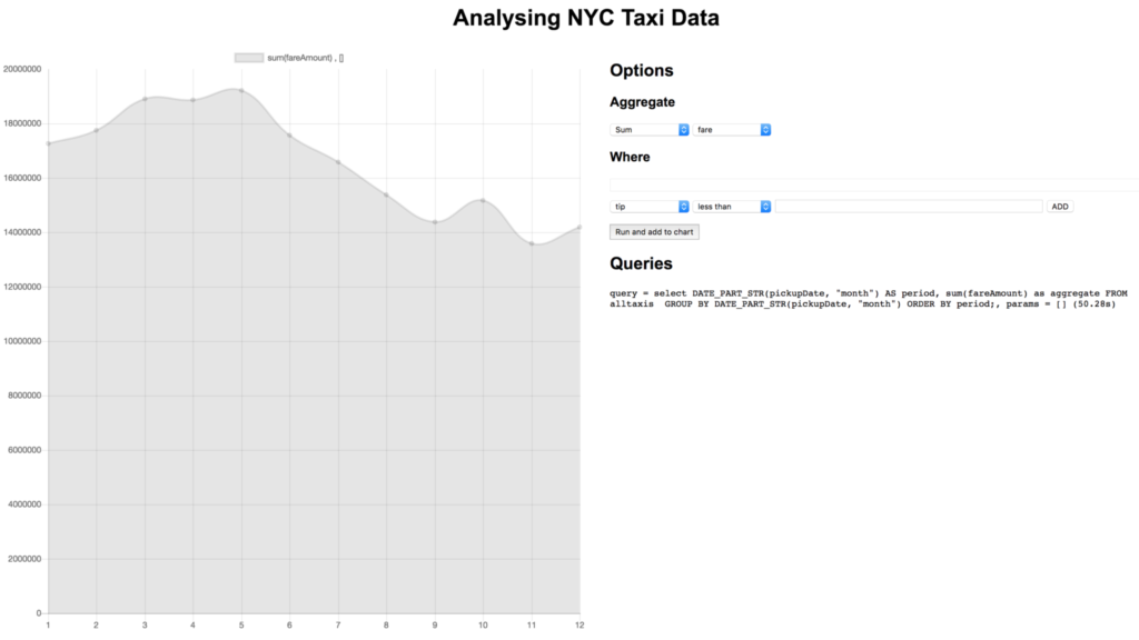
Using the frontend we can easily try out different aggregates for different fields, apply where clauses and drill into the data to get a more granular view on things. For example we probably want to know in which month taxis generated the most money:
Let’s dig into this by clicking on the dot corresponding to May:
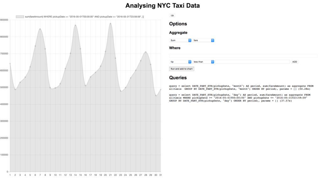
It looks like the most money is generated on weekends, that makes sense. As it’s nice in May and weekends are most popular maybe most trips are multiple passengers going to see the sights together?
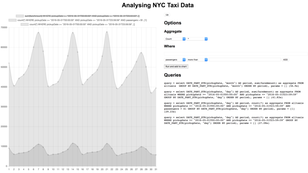
Doesn’t look like it! There are lots of other comparisons that we could make, like fares vs tips or the number of journeys vs number of journeys with no tips. This dataset also has location data so we could do things like create heatmaps of pickup locations.
Conclusion
In this example, we walked through how a simple query, which might even be ad-hoc, can be used to quickly analyze a dataset with a variety of metrics, all without requiring the creation of indexes. Couchbase Analytics will add this great capability to the Couchbase platform when made generally available. Golang developers have access now through the 6.0 beta.
We’d love your feedback! Please download Couchbase Server 6.0 beta today and try the updated Couchbase Analytics. We’ll be watching for your comments at www.couchbase.com/forums/ on anything from analytics to the Go SDK.